Linear Mixed Effects Models
- 9th May 2025
- Posted by: Breige McBride
- Category: Bioinformatics
In clinical trials it is common to collect samples from trial participants at multiple time points, resulting in repeated measures data. Statistical methods used to analyse this data must account for the correlation between measurements from the same participant. Below we describe linear mixed effects modelling to assess repeated measures data.
Linear mixed effects models comprise fixed effects and random effects, which capture non-independent data points. In a clinical trial, fixed effects model non-random parameters of the study design (e.g. treatment group or sex of a trial participant). In studies that collect samples longitudinally, the patient effect introduced by the presence of repeated measures is something that cannot be controlled and is treated as random. A study may comprise more than one random effect, and random effects can be nested. For example, in mouse clinical trials (Guo et al. BMC Cancer, 2019) where animals are implanted with patient tumours which are then harvested and re-implanted, the random effects come from the original patient cohort as well as mice from subsequent passages.
Linear Mixed Effect Model Example
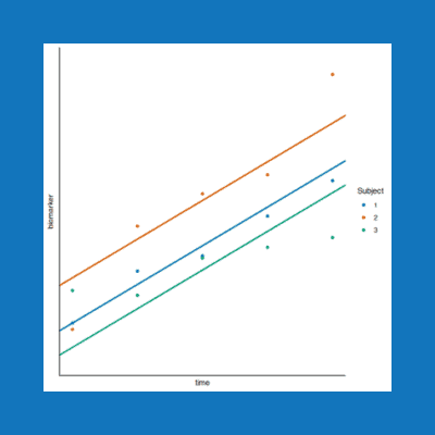
Biomarker data from a clinical trial with repeated measures
In a clinical trial with three treatment arms, with samples collected at three time points post treatment, biomarker abundance can be expressed as a function of treatment and time. The interaction between treatment and time is modelled as it is expected that the effect of time point on biomarker abundance is dependent on treatment arm. The following linear regression models the fixed effects of this example:
biomarker ~ intercept + treatment + time + treatment:time
This model violates the independence assumption of linear models, as each trial participant (subject) has three samples. The random subject effect is accounted for as follows:
biomarker ~ intercept + treatment + time + treatment:time + (1|subject)
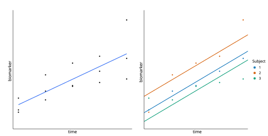
This equation uses the R syntax, where “(1 |subject)” instructs the model to allow an intercept per subject. In other words, the model allows the baseline biomarker value to differ per patient. The difference between a fixed effects model and a random effects model with an intercept per subject is illustrated in Figure 1, below.
Understanding the Results
Implementing the above model is only the first step. The next step is understanding the model results. The following description of the model output, while general, is based on implementing this model using the lmer function from the lme4 R package (Bates et al., 2015, Journal of Statistical Software).
First, as instructed, the model will return an intercept per patient as well as the standard deviation for the random effect, which indicates how much variability in biomarker abundance is due to the subject effect. The model will also return a coefficient (effect size) and associated statistics for each of the fixed effects. Note that the model intercept is the average value of the per patient intercepts.
While the fixed effects coefficients give us information about specific differences between treatments and time points (in relation to the reference levels of each variable), they only tell part of the story. To determine the average treatment effect on biomarker abundance for different treatment arms, we can calculate the estimated marginal means (also known as least-squares means) at each time point using the emmeans function in the emmeans R package. Using the same function, it is then possible to formulate contrasts to determine whether the treatment effects are significantly different between treatment groups.
Alternative Model
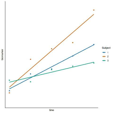
An alternative random effects model could be implemented to allow for an intercept and a slope per subject (Figure 2, below). While it may seem more realistic to allow the treatment effect to differ per subject, it is not always possible to introduce more complexity to the model due to the study design. For example, if there is a random intercept and slope per subject, this doubles the number of random effects to be estimated, which may be greater than the number of points in the data set.
In addition, the model described above can be extended to include further fixed effects and interactions terms. For example, baseline (pre-treatment) biomarker value could be included as a fixed effect to account for baseline differences per subject.
Linear Mixed Effects Models – Tips
R packages other than lmer are available to implement linear mixed effects models (e.g. the nlme R package). The limma modelling framework (Ritchie et al., 2015, Nucleic Acids Research) accounts for repeated measures by modelling the correlations between samples using the duplicateCorrelation function. However, this is only suitable when there is a single random effect.
It is also possible to model a binary response variable as a function of one or more predictor variables from repeated measures data. The glmer function from the lme4 R package, with the parameter family set to binomial, can be used to fit a mixed effects logistic regression model. In this case, the fixed-effect and random-effect coefficients should be interpreted as changes in log-odds.
There are other methods to assess repeated measures data. For example, the repeated measures analysis of variance (ANOVA) method. However, if a subject does not have data available from all time points in a clinical trial, the subject will be dropped from the analysis. Incomplete data is not an issue for linear mixed effects models.
Overall, linear mixed effects modelling offers a highly flexible framework to capture the relationships between clinical study design parameters and the response variable of interest, while accounting for patient-to-patient variation. If you would like the support of expert bioinformatics team to leverage linear mixed effects modelling in you clinical trial, simply use the form below to contact us and we will be happy to help!
See Also:
How Bioinformatics Can Support Your Clinical Trial
Tool Selection for Cellular Deconvolution
Target Triage: Faster, Smarter, Drug Target Selection
